From Practitioner to Certified: My AI Engineering for Developers Journey
I recently earned the AI Engineering for Developers Associate certification from DataCamp. But here’s the thing—I was already building LLM-integrated applications before I enrolled.
So why take the course? And was it worth it?
Absolutely.
Already in the Game
Before starting this career path, I had been building AI-powered systems with both Python and JavaScript. I was familiar with prompt engineering, had experimented with various LLM APIs, and had even drawn inspiration from some of the best documentation in the industry—particularly Anthropic Claude’s guidelines on structured system prompting.
I wasn’t starting from zero. But I knew there were gaps in my knowledge, especially around production-grade practices and the deeper mechanics of how these systems work under the hood.
Why This Path Aligned Perfectly
The AI Engineering for Developers career track wasn’t just theoretical—it mapped directly to the work I was already doing. It validated some of my existing practices while introducing concepts I hadn’t fully explored.
The curriculum covered exactly what a modern AI engineer needs:
LLM Application Architecture: Different methods and patterns for building robust LLM-integrated applications
Embeddings Deep Dive: Finally understanding vector representations at a fundamental level
LLMOps Workflows: The entire lifecycle of LLM applications in production
HuggingFace Ecosystem: Discovering the platform from a professional, production-ready perspective
LangChain & LangGraph: Building sophisticated agent systems
The LLMOps Revelation
One of the most valuable sections was the deep dive into LLMOps and how it differs from traditional MLOps.
While MLOps focuses on model training, versioning, and deployment pipelines, LLMOps introduces entirely new challenges:
Understanding this distinction has fundamentally changed how I think about deploying and maintaining my AI applications.
HuggingFace: A Professional Perspective
I had used HuggingFace before, but mostly for quick model downloads. This path changed that entirely.
Learning to navigate the ecosystem professionally—understanding model cards, leveraging the Transformers library effectively, and integrating HuggingFace into production workflows—opened up new possibilities for my projects.
My Favorite Part: LangChain & LangGraph
This was the section I was most excited about, and it didn’t disappoint.
I’ve been using LangChain and LangGraph extensively in my projects. They’re crucial components of my development toolkit. The course reinforced best practices and introduced patterns I hadn’t considered:
Building proper ReAct (Reasoning + Acting) agent systems
Architecting multi-agent RAG systems that actually scale
Connecting LLMs to external tools, including MCP (Model Context Protocol) integrations
These frameworks make building sophisticated AI systems a much more pleasant experience. The abstraction they provide—while maintaining flexibility—is exactly what production applications need.
The career track included optional bonus projects designed to prepare you for the certification exam. I completed all of them.
Were they challenging? Yes.
Were they worth it? Absolutely.
These projects forced me to apply concepts in ways I hadn’t before. They exposed edge cases and gotchas that I might have missed in a real-world scenario. By the time I sat for the certification exam, I felt genuinely prepared.
Not Just Basics
Here’s what surprised me most: this wasn’t a beginner course pretending to be advanced.
The intermediate courses within the path went deep. While I was already familiar with concepts like few-shot prompting and basic prompt engineering, the path pushed further:
Production-grade error handling for LLM applications
The Certification
After completing the career path and all bonus projects, I passed the AI Engineering for Developers Associate certification exam.
But more valuable than the credential itself is the structured knowledge I gained. The certification validated what I knew while filling in the gaps I didn’t know I had.
What’s Next
This journey has reinforced my direction. AI engineering isn’t just about making API calls—it’s about building reliable, maintainable, and scalable systems that leverage the power of large language models.
The skills from this path are already being applied across my projects. From agentic workflows to RAG pipelines, the depth of understanding I gained continues to pay dividends.
If you’re already working with LLMs and wondering whether a structured learning path is worth it—it is. Sometimes you need that formal structure to connect the dots between what you know and what you should know.
Check out my projects and contributions on GitHub.
Mastering AI Engineering: From Theory to Production
I recently finished a deep dive course on AI Engineering, focusing on moving beyond simple “chat” interfaces to building robust, engineering-grade applications. It’s been a game-changer. The transition from using LLMs to engineering them requires a shift in mindset—from “asking questions” to “designing systems.”
Here is how I’m applying these advanced concepts to my own projects, like Kaelux-Automate and ModelForge.
Under the Hood: Parameter Tuning
One of the first things I learned is that default API settings are rarely optimal for complex logic. In my ModelForge project, I don’t just call the endpoint; I tune the parameters to control the “creativity” vs. “determinism” trade-off.
For example, when integrating the Gemini 2.0 Flash model, I explicitly set the temperature and topP values to ensure the model follows instructions without hallucinating wild geometry:
// From ModelForge/lib/gemini.tsexport async function generateGeminiResponse({ messages, temperature = 0.4, // Lower temperature for more deterministic code generation topP = 0.8, // ...})
By lowering the temperature to 0.4, I force the model to be more conservative, which is critical when generating Python scripts that must execute inside Blender without errors.
Advanced Prompt Engineering Patterns
The course reinforced several patterns I had started using but now understand deeply.
1. System Prompts & Context
It’s not enough to just send a user message. You need to set the “persona” and boundaries. In ModelForge, I build a dynamic system prompt that injects guidelines and tool definitions:
// From ModelForge/lib/orchestration/prompts.tsexport function buildSystemPrompt() { return [REACT_GUIDELINES, TOOL_DESCRIPTIONS, FEW_SHOT_EXAMPLES].join("\n\n")}
This ensures the model knows exactly what tools it has (like get_scene_info or execute_code) and how to use them before it even sees the user’s request.
2. Chain-of-Thought (CoT) & ReAct
One of the most powerful techniques is forcing the model to “think” before it acts. In my system prompts, I explicitly instruct the model to follow a ReAct (Reason + Act) loop:
“Thought: Reflect on the user’s intent… Action: Invoke tool…”
This imposes a “Chain of Thought” structure, preventing the model from jumping to incorrect conclusions.
3. Few-Shot Learning
Theory says “give examples,” and practice proves it works. I tried 0-shot prompting for complex Blender scripts, and it failed often. By providing Few-Shot examples—actual snippet pairs of User Input -> Python Code—I significantly improved the reliability of the output.
4. Self-Consistency
A new technique I learned and am now experimenting with is Self-Consistency. Instead of taking the first answer, you prompt the model multiple times (generating multiple “chains of thought”) and pick the most consistent answer. This is computationally more expensive but incredibly useful for high-stakes logic limits.
The Future: LangChain
The natural next step is LangChain, which takes these manual patterns (Code Owners, System Prompts, Message History) and abstracts them into reusable chains. I’ve already started exploring this, but my hands-on work with raw API calls gave me the intuition to know what LangChain is actually doing under the hood.
I highly recommend digging into these engineering practices. Don’t just chat with the bot—build the system that controls it.
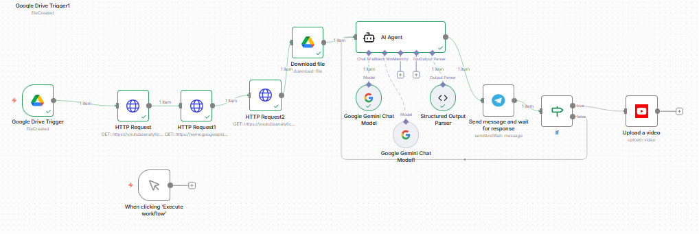
Building a Smart YouTube Automation Agent with n8n and Gemini
I spent the entire day building a comprehensive YouTube automation workflow in n8n from scratch. It was one of those days where “just connecting an API” turns into a deep dive into OAuth scopes and raw HTTP requests.
The Cloud Credentials Maze
Despite being very familiar with Google Cloud—hosting multiple projects, instances, and even my self-hosted n8n instance there—setting up the credentials for this was still a mess.
It wasn’t just about getting a Client ID and Secret. It was about configuring the consent screen, ensuring the right scopes were enabled for both the YouTube Data API and the Analytics API, and tweaking the redirect URIs until the handshake finally worked. If you think experienced devs don’t struggle with IAM and OAuth every time, you’re wrong.
The Limitation: n8n Native Nodes
My initial plan was simple: use the built-in n8n YouTube nodes. I quickly hit a wall.
The native nodes are great for basic tasks like “Upload Video” or “Get Channel Statistics,” but they hide the granular data. I needed deep analytics—specifically watch time and average view duration. These are the metrics that actually drive channel growth, not just raw view counts.
The Solution? I had to abandon the comfort of the pre-built nodes and build my own API calls using HTTP Request nodes. This gave me direct access to the youtubeAnalytics endpoint, allowing me to fetch the specific reports I needed.
The AI Brain: Gemini 3 Pro
The workflow doesn’t just “post and forget.” It acts as an intelligent agent.
Trigger: It watches a specific Google Drive folder for a ready-to-upload video file.
Analysis: It scrapes my channel’s recent performance data using those custom HTTP requests.
Decision: Instead of just posting at a “standard” time or targeting a high-traffic region, I feed this data into Gemini 3 Pro.
The AI analyzes the watch time and retention trends to determine the absolute best upload slot. It also strictly enforces a “Max 1 Post Per Day” policy to keep the algorithm happy, checking my recent schedule to ensure we don’t spam the channel.
It was a long process of trial and error, but the result is a workflow that doesn’t just automate the action of uploading, but automates the intelligence behind the scheduling.
The 10-Second Barrier: My Quest for Professional AI Video Generation
I’ve been on a mission to find the best tools for generating professional marketing videos using the latest AI models. With heavyweights like OpenAI’s Sora and Google’s Veo hitting the market, you’d think we’d be in a golden age of limitless video creation.
But after extensive testing, I’ve hit a frustrating reality: The 10-Second Barrier.
The Problem: Short Attention Spans (Literally)
Whether you’re using Sora or Veo, you are generally capped at generating videos of just 8 to 10 seconds.
For a TikTok clip, that might be fine. For professional marketing? It’s a nightmare. The biggest challenge isn’t just the length—it’s the difficulty of seamlessly extending or transitioning from one generation to another without the quality falling apart.
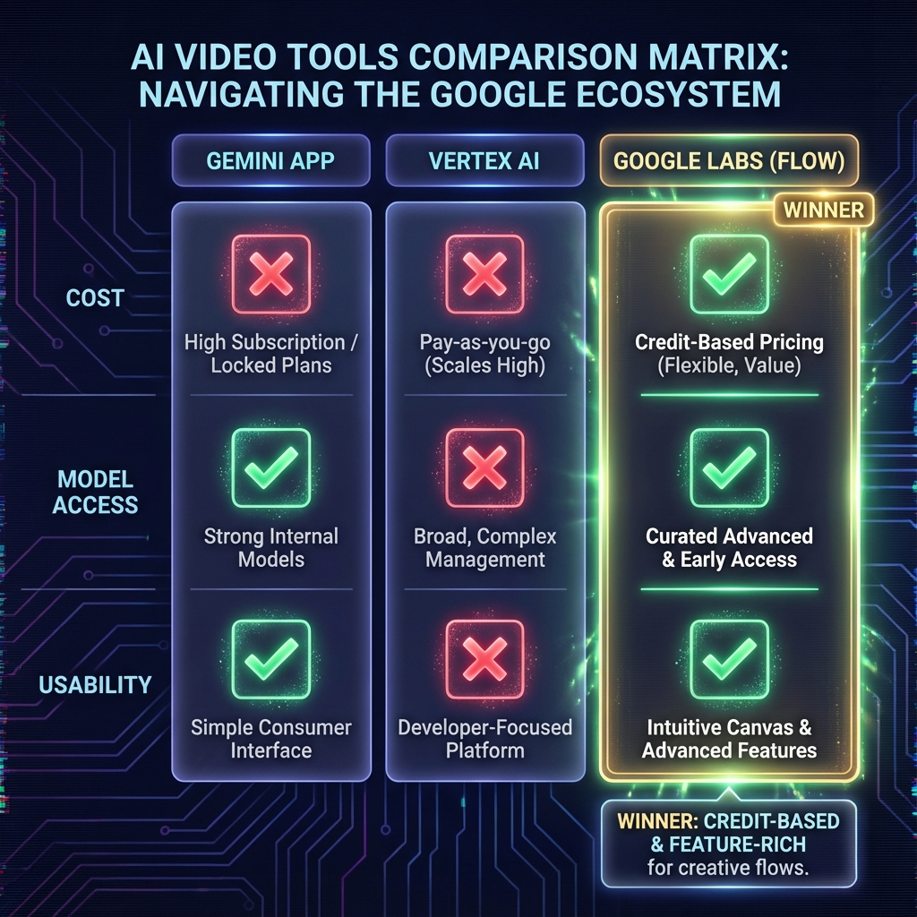
The Platform Gauntlet
I tested Google’s Veo models across every available interface to find a workaround. Here is what I found:
1. The Gemini App
Verdict: Avoid for professional work.
It’s great for quick, fun experiments, but it strictly enforces the 8-second limit. There are no advanced controls for extension or editing.
2. Google AI Studio
Verdict: Currently broken.
As of today, the model preview environment seems buggy. I found myself stuck with the older Veo 2.0 model unless I built a custom app using the Veo 3.1 preview API. It’s not a ready-to-use creative studio.
3. Vertex AI (Model Garden)
Verdict: Powerful but expensive.
Vertex AI offers more control, but it requires using your Google Cloud API key.
Cost: It gets extremely expensive very quickly if you’re iterating on multiple videos.
Bugs: I encountered output errors when trying to use the “Extend Video” feature.
Limitations: Surprisingly, you are often limited to extending videos only with the older Veo 2.0 model, which doesn’t even generate audio.
The Solution: Google Labs (Flow)
After hitting dead ends everywhere else, I finally arrived at a conclusion. The most effective environment right now is Google Labs Flow.
Why It Wins
Instead of burning through your API key, Flow uses a credit system (based on your Google AI subscription).
Newest Models: It gives you access to the latest Veo capabilities.
“Jump To” Feature: This is basically a more efficient way to extend videos, allowing you to navigate to a specific frame and generate the next segment.
Reasonable Pricing: The credit usage feels fair compared to raw API costs.
The Critique
It’s not perfect. The “Extend Video” feature is still hit-or-miss, and quality can degrade. But compared to the broken previews of AI Studio or the high costs of Vertex, Google seems to have put the most effort into making Flow a usable product for creators.
Conclusion
We aren’t quite at the “text-to-movie” stage yet. The 8-second limit is a hard constraint that requires clever editing and patience to work around. But if you’re looking to experiment without breaking the bank (or your code), Google Labs Flow is currently your best bet.
I’ll keep experimenting with this platform and update this post as the tools evolve.
Docker Foundations: From Containers to Kubernetes
I’ve recently completed the Docker Foundations Professional Certificate, and it has completely changed how I approach software development and deployment. In this post, I want to share what I’ve learned—from the basics of containers to the complexity of Kubernetes—and show you how I’m already applying these concepts in my real-world projects.
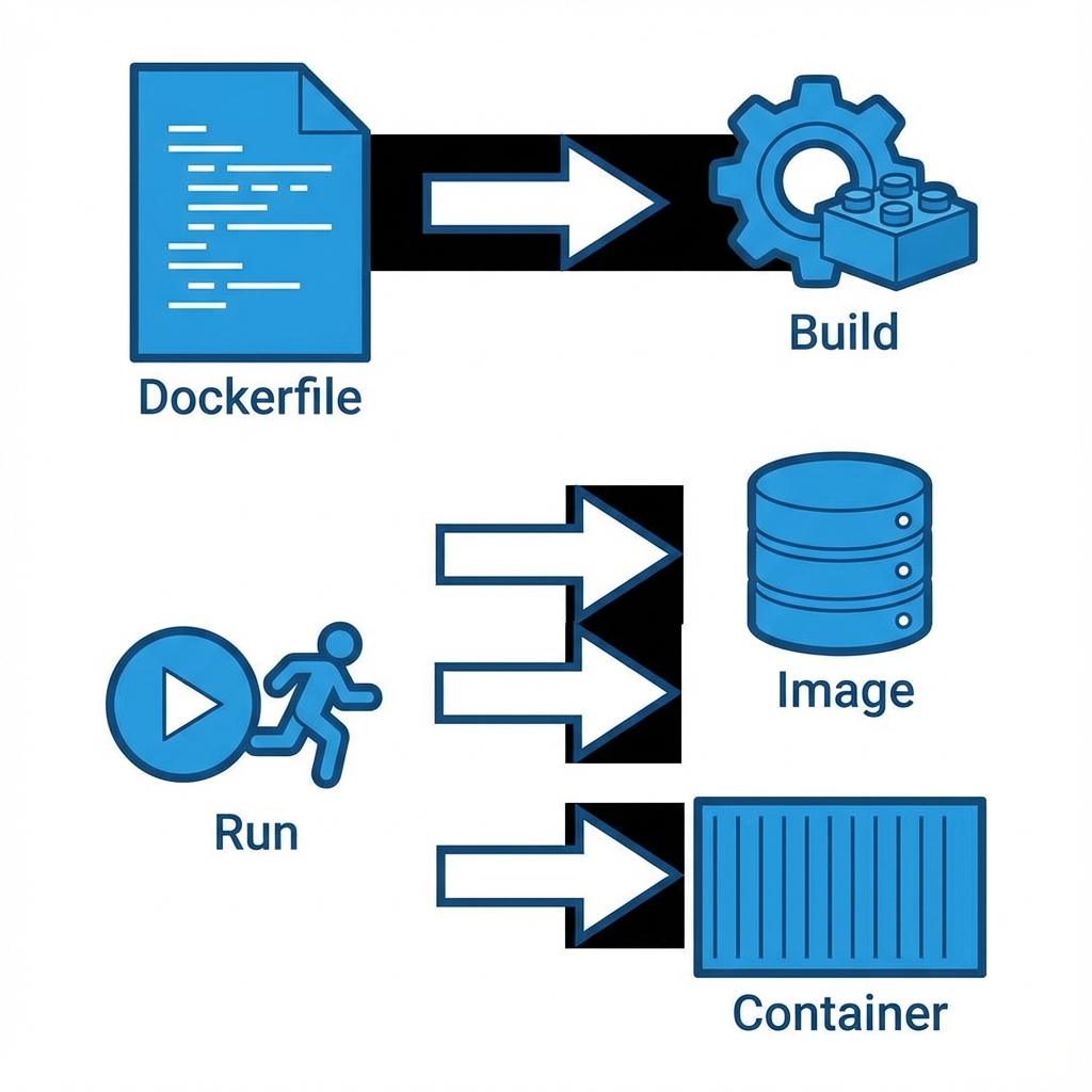
The Docker Workflow
Before diving into the code, it’s essential to understand the core workflow. Docker isn’t just about “running containers”; it’s a pipeline for building consistent environments.
1. The Dockerfile
Everything starts with a Dockerfile. This is the blueprint. In my learning repository, docker-your-first-project-4485003, I learned that a Dockerfile is essentially a script of instructions.
# Example from my learning pathFROM node:14-alpineWORKDIR /appCOPY package*.json ./RUN npm installCOPY . .EXPOSE 3000CMD ["npm", "start"]
2. Building the Image
The docker build command takes that blueprint and creates an Image. An image is a read-only template. It includes your code, libraries, dependencies, and tools. It’s immutable—once built, it doesn’t change.
3. Running the Container
When you run an image, it becomes a Container. This is the live, running instance. You can have multiple containers running from the same image, completely isolated from each other.
Advanced Management
Learning the basics was just the start. The certificate also covered how to manage these containers efficiently in a production-like environment.
Data Persistence with Volumes
One of the first “gotchas” with Docker is that data inside a container is ephemeral. If the container dies, the data dies. I learned to use Volumes to persist data.
docker run -v my_volume:/var/lib/mysql mysql
This maps a storage area on my host machine to the container, ensuring my database doesn’t get wiped out on a restart.
Efficient Runtime & Pruning
Over time, building images leaves behind “dangling” layers and stopped containers. I learned the importance of keeping the environment clean to save disk space:
# The magic command to clean up unused objectsdocker system prune
Orchestration: Compose & Kubernetes
Running one container is easy. Running a web server, a database, and a cache all together? That’s where Docker Compose comes in.
In my projects, I use docker-compose.yml to define multi-container applications. It allows me to spin up my entire stack with a single command: docker-compose up.
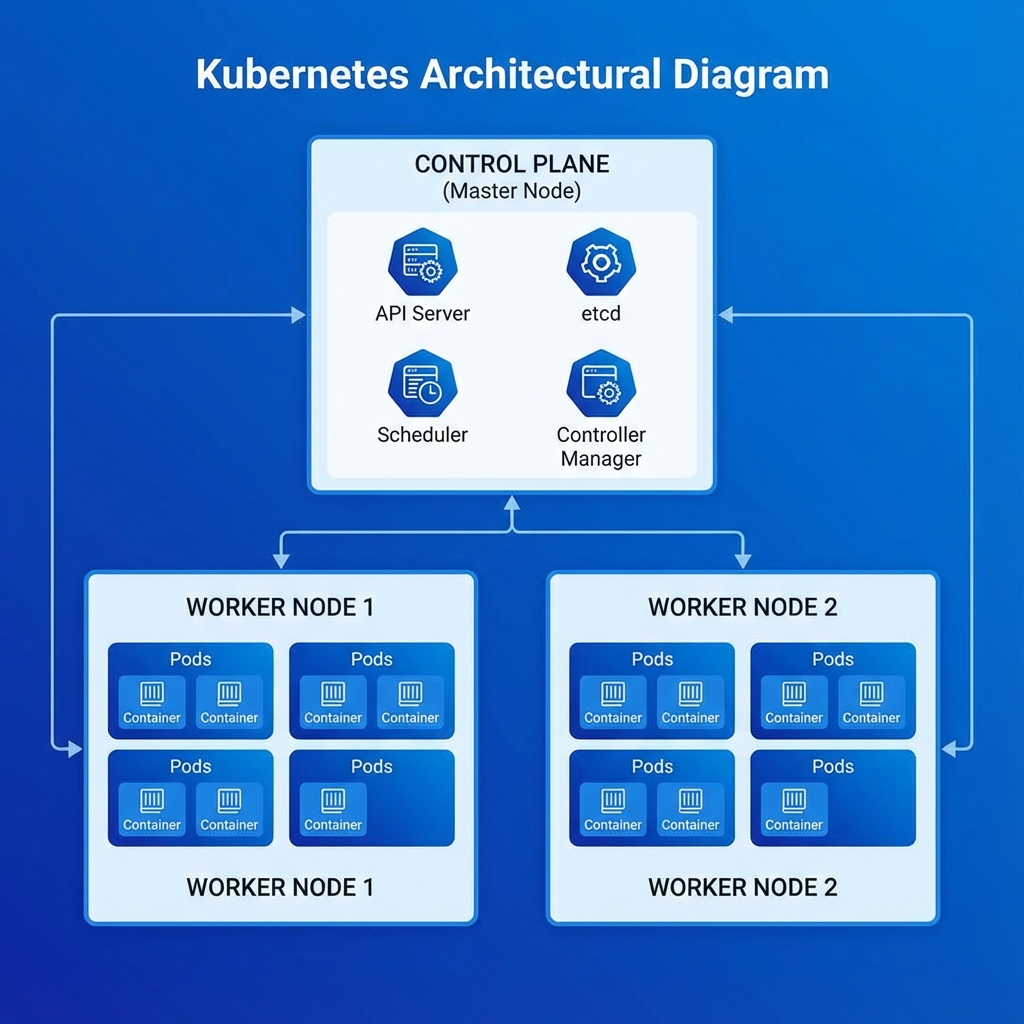
Scaling with Kubernetes
But what happens when you need to scale across multiple servers? That’s where Kubernetes (K8s) enters the picture.
Kubernetes takes container management to the next level. It uses a Control Plane to manage Worker Nodes, which in turn run Pods (groups of containers). It handles:
Auto-scaling: Adding more pods when traffic spikes.
I’m not just learning this in theory; I’m using it. In my project, Kaelux-Automate, Docker is critical.
Why Docker for Automation?
This project involves complex workflows with n8n, which connects to various services including Pinecone (a Vector Database) for AI memory.
Consistency: I can run the exact same n8n version on my laptop and my server. No “it works on my machine” bugs.
Isolation: The AI components and the workflow engine run in separate containers, ensuring that a heavy process in one doesn’t crash the other.
Vector DB Integration: Connecting to Pinecone requires secure environment variable management, which Docker handles gracefully through .env files passed at runtime.
Orchestration with ModelForge
Another project where I rely heavily on Docker is ModelForge, my AI-powered Blender assistant.
Here, I use Docker Compose to orchestrate multiple services:
The main Electron application.
A local database (PostgreSQL) for asset management.
The AI orchestration layer.
Using Compose allows me to define the entire stack in a single docker-compose.yml file, making it incredibly easy for other developers to spin up the project with a single command: docker-compose up.
Conclusion
Docker has become a foundational tool in my developer toolkit. Whether I’m spinning up a quick test environment for a new library or deploying a complex AI automation system, the ability to containerize applications ensures they run reliably, everywhere.
My GH-900 Journey: Failing, Learning, and Mastering GitHub
I have a confession to make: I failed my first attempt at the GitHub Foundations (GH-900) exam.
Despite having hands-on experience with Git and taking a dedicated DataCamp course, I walked out of that first exam humbled. But looking back, failing was the best thing that could have happened to my development career.
The First Attempt: A Reality Check
I went in confident. I knew how to commit, push, pull, and manage branches. I thought I was ready.
But the exam threw curveballs I wasn’t expecting. It wasn’t just about “using Git”; it was about the entire GitHub ecosystem.
The questions drilled deep into:
GitHub Enterprise: Management, billing, and organization structures I had never touched as a solo dev.
GitHub Actions: Specific syntax and workflow configurations that went far beyond simple CI scripts.
I realized my knowledge was “practical” but narrow. I knew how to code, but I didn’t know how to administer and automate at an enterprise scale.
The Rabbit Hole: Going Deep
After the failure, I didn’t just want to pass; I wanted to master it. I pivoted to the official Microsoft Learn documentation and decided to explore every single feature GitHub offers.
I built multiple projects solely to test features I’d ignored:
Configuring complex Branch Protection Rules.
Setting up Code Owners to enforce review policies.
Diving into GitHub Projects for agile management.
Writing intricate GitHub Actions workflows.
The Second Attempt: Mastery
When I sat for the exam the second time, it was a completely different experience. I didn’t just know the answers; I understood the why behind them. I passed with an excellent score.
However, I still have one critique.
The Missing Piece: The Command Line
Ironically, the one area where I was strongest—the Git CLI—was barely present.
The exam focuses heavily on the web interface and platform features. It asks about button clicks in settings menus but skips the nitty-gritty of git rebase -i or git cherry-pick. If you’re a command-line warrior, don’t expect that to save you here.
What the Exam Actually Covers
If you’re planning to take GH-900, know that “Foundations” is a bit of a misnomer. It covers a lot of ground.
1. GitHub Actions (The Big One)
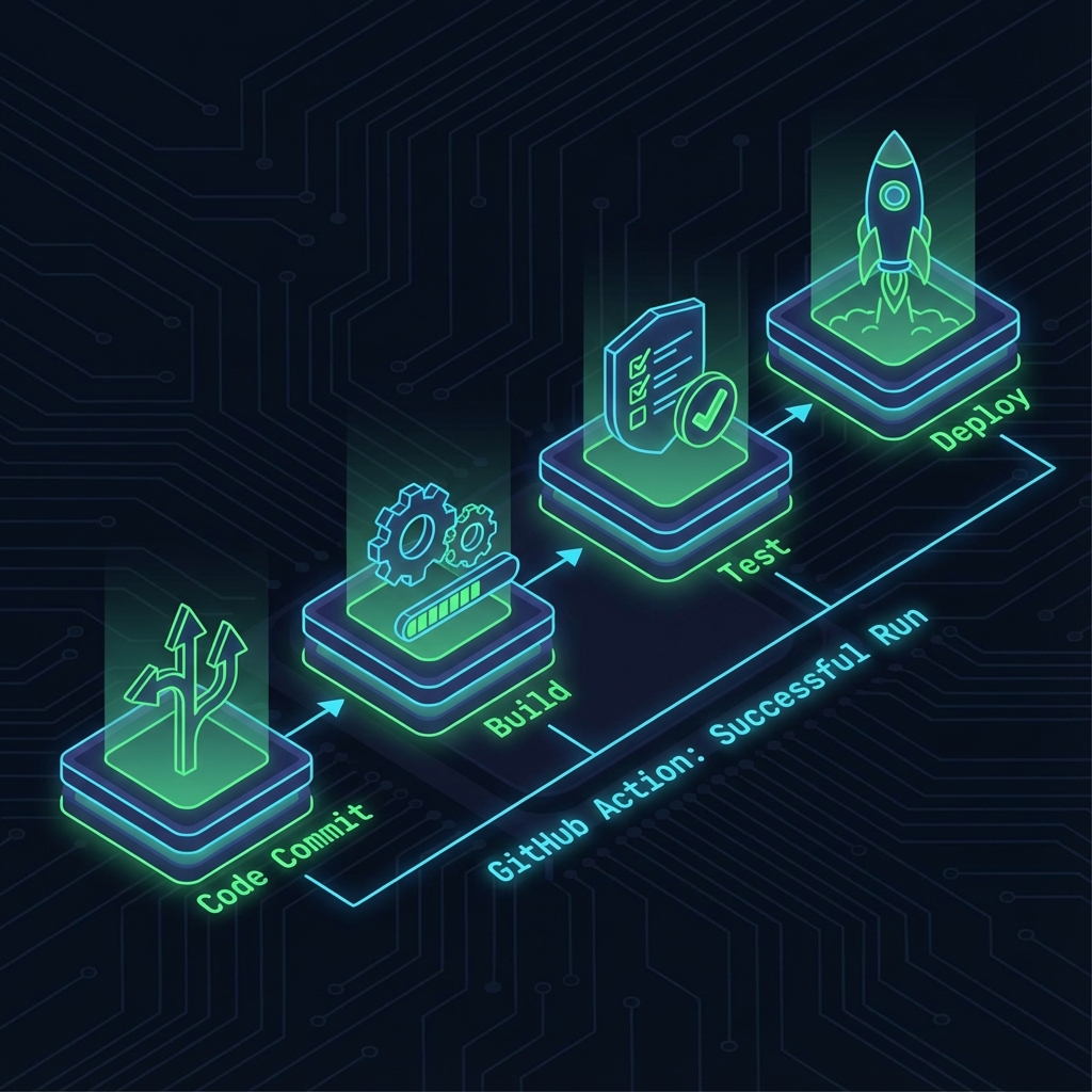
You need to understand CI/CD pipelines inside and out.
It’s not enough to know what it is; you need to know how to read a YAML workflow file, understand triggers (on: push, on: pull_request), and manage secrets.
2. GitHub Enterprise & Security
Expect questions on:
SAML SSO: How authentication works in big orgs.
Dependabot: How to configure automated security updates.
Secret Scanning: What happens when you accidentally commit an API key.
Conclusion
Failing the GH-900 pushed me down a rabbit hole that expanded my skills far beyond just “version control.” The extra knowledge I gained—especially in automation and project management—has been invaluable in my recent projects.
If you fail, don’t be discouraged. Use it as a roadmap for what you still need to learn. The destination is worth it.
Machine Learning Fundamentals: From Zero to Understanding Modern AI
Machine Learning (ML) has become one of the most transformative technologies of our time. From recommendation systems on Netflix to self-driving cars, ML is everywhere. But what actually is machine learning? How does it differ from traditional programming? And how did we go from simple algorithms to the powerful Large Language Models (LLMs) like GPT-4 and Claude that can hold conversations and write code?
In this post, I’m documenting everything I learned about machine learning fundamentals — the concepts, algorithms, methodologies, and the step-by-step pipeline that takes raw data and turns it into intelligent systems.
My Learning Environment: Python, Anaconda & GitHub Codespaces
Before diving into the concepts, let me share the setup I used for this learning journey.
Why Python?
Python is the de facto language for machine learning. Its simplicity, combined with powerful libraries like NumPy, Pandas, Scikit-learn, TensorFlow, and PyTorch, makes it the perfect choice.
Why Anaconda?
Anaconda is a distribution of Python designed specifically for data science and machine learning. It comes pre-packaged with:
Pre-installed libraries: NumPy, Pandas, Matplotlib, Scikit-learn, and more
# Creating a new conda environment for MLconda create -n ml-fundamentals python=3.11conda activate ml-fundamentals# Installing essential ML packagesconda install numpy pandas scikit-learn matplotlib seaborn jupyter
Why GitHub Codespaces?
GitHub Codespaces provides a complete, configurable dev environment in the cloud. This means:
No local setup headaches — everything runs in a browser
Consistent environment — same setup every time
Powerful compute — access to machines with more RAM/CPU than my laptop
Pre-configured containers — I used a Python/Anaconda devcontainer
This combination allowed me to focus on learning rather than fighting with installations.
What is Machine Learning?
At its core, machine learning is a subset of artificial intelligence that enables systems to learn and improve from experience without being explicitly programmed.
Traditional Programming vs Machine Learning
Traditional Programming
Machine Learning
Input: Data + Rules
Input: Data + Expected Output
Output: Results
Output: Rules (Model)
Human writes logic
Machine discovers logic
Explicit instructions
Pattern recognition
In traditional programming, you tell the computer exactly what to do:
# Traditional: Explicit rulesdef is_spam(email): if "free money" in email.lower(): return True if "click here" in email.lower(): return True return False
In machine learning, you give examples and let the computer figure out the rules:
# ML: Learn from examplesfrom sklearn.naive_bayes import MultinomialNB# Train on thousands of labeled emailsmodel = MultinomialNB()model.fit(email_features, labels) # labels: spam or not spam# Model discovers its own rulesprediction = model.predict(new_email_features)
Machine Learning vs Artificial Intelligence vs Deep Learning
These terms are often used interchangeably, but they have distinct meanings:
The algorithm learns by interacting with an environment and receiving rewards or penalties.
Analogy: Training a dog with treats — good behavior gets rewards, bad behavior doesn’t.
# Conceptual example (simplified)# Agent learns to play a game by trial and errorfor episode in range(1000): state = environment.reset() while not done: action = agent.choose_action(state) next_state, reward, done = environment.step(action) agent.learn(state, action, reward, next_state) state = next_state
Applications:
Game playing (AlphaGo, Chess engines)
Robotics
Autonomous vehicles
Resource management
Classification vs Regression
Within supervised learning, there are two main problem types:
Classification
Predicting a category or class label.
Problem
Output
Is this email spam?
Yes / No (Binary)
What digit is this?
0-9 (Multi-class)
What objects are in this image?
Multiple labels (Multi-label)
from sklearn.tree import DecisionTreeClassifier# Classification: Predict if a customer will churn (Yes/No)X = [[25, 12, 50000], [45, 36, 80000], [35, 6, 45000]] # age, months_customer, spendy = ['No', 'No', 'Yes'] # Churned?clf = DecisionTreeClassifier()clf.fit(X, y)new_customer = [[30, 3, 30000]]prediction = clf.predict(new_customer) # 'Yes' or 'No'
from sklearn.preprocessing import StandardScaler, MinMaxScaler# Standardization (mean=0, std=1) - good for most algorithmsscaler = StandardScaler()X_scaled = scaler.fit_transform(X)# Normalization (0-1 range) - good when you need bounded valuesminmax = MinMaxScaler()X_normalized = minmax.fit_transform(X)
Train-Test Split
from sklearn.model_selection import train_test_splitX_train, X_test, y_train, y_test = train_test_split( X, y, test_size=0.2, # 20% for testing random_state=42, # Reproducibility stratify=y # Maintain class distribution (for classification))
Stage 4: Modeling
Goal: Train machine learning models on prepared data.
from sklearn.ensemble import RandomForestClassifierfrom sklearn.linear_model import LogisticRegressionfrom sklearn.svm import SVC# Define models to trymodels = { 'Logistic Regression': LogisticRegression(max_iter=1000), 'Random Forest': RandomForestClassifier(n_estimators=100, random_state=42), 'SVM': SVC(kernel='rbf', random_state=42)}# Train and evaluate each modelfor name, model in models.items(): model.fit(X_train, y_train) train_score = model.score(X_train, y_train) test_score = model.score(X_test, y_test) print(f"{name}: Train={train_score:.4f}, Test={test_score:.4f}")
Hyperparameter Tuning
from sklearn.model_selection import GridSearchCV, RandomizedSearchCV# Grid Search - exhaustive search over parameter gridparam_grid = { 'n_estimators': [100, 200, 300], 'max_depth': [10, 20, 30, None], 'min_samples_split': [2, 5, 10]}grid_search = GridSearchCV( RandomForestClassifier(random_state=42), param_grid, cv=5, # 5-fold cross-validation scoring='accuracy', n_jobs=-1 # Use all CPU cores)grid_search.fit(X_train, y_train)print(f"Best parameters: {grid_search.best_params_}")print(f"Best score: {grid_search.best_score_}")
Stage 5: Evaluation
Goal: Assess model performance using appropriate metrics.
This was the most fascinating part of my learning — understanding how models like GPT-4, Claude, and Llama actually work.
The Evolution to Transformers
Before transformers, we had:
RNNs (Recurrent Neural Networks): Processed sequences one word at a time
LSTMs (Long Short-Term Memory): Better at remembering long-term dependencies
Attention Mechanisms: Allowed models to “focus” on relevant parts of input
Then in 2017, the paper “Attention Is All You Need” introduced the Transformer architecture, which changed everything.
Key Concepts in Transformers
1. Self-Attention Mechanism
Self-attention allows each word to “look at” all other words in a sequence and determine their relevance.
Query: "The cat sat on the mat because it was tired"
                                        ↑
                          "it" attends to "cat" (not "mat")
The model learns that “it” refers to “cat” by attending to context.
2. Positional Encoding
Since transformers process all words simultaneously (not sequentially), they need a way to understand word order. Positional encodings add this information.
3. Multi-Head Attention
Instead of one attention mechanism, transformers use multiple “heads” that can attend to different aspects (syntax, semantics, etc.) simultaneously.
4. Feed-Forward Networks
After attention, each position passes through a feed-forward network independently.
Self-Supervised Learning: The Secret Sauce
Modern LLMs are trained using self-supervised learning — they create their own labels from unlabeled data.
For GPT-style models (Decoder-only):
Task: Predict the next word
Input: "The quick brown fox jumps over the lazy"Target: "dog"
The model sees trillions of such examples and learns language patterns.
For BERT-style models (Encoder-only):
Task: Masked Language Modeling
Input: "The quick brown [MASK] jumps over the lazy dog"Target: "fox"
The Scale of Modern LLMs
What makes GPT-4 and similar models so powerful?
Factor
Impact
Parameters
Billions to trillions of learnable weights
Training Data
Trillions of tokens from the internet
Compute
Thousands of GPUs for months
Architecture
Optimized transformer variants
Fine-tuning
RLHF (Reinforcement Learning from Human Feedback)
The Training Pipeline for LLMs
Pre-training: Self-supervised learning on massive text data
Model learns grammar, facts, reasoning patterns
Expensive: millions of dollars in compute
Supervised Fine-Tuning (SFT): Train on human-written examples
High-quality prompt-response pairs
Teaches the model to be helpful
RLHF (Reinforcement Learning from Human Feedback):
Humans rank model outputs
Train a reward model on these preferences
Use RL to optimize the model to produce highly-ranked outputs
This is just the beginning. My next steps in the ML journey:
Deep dive into transformers — Implement attention from scratch
Explore MLOps — Model deployment, monitoring, and versioning
Computer Vision — CNNs and image classification
Natural Language Processing — Fine-tuning LLMs for specific tasks
Build real projects — Apply these concepts to solve actual problems
Machine learning is a vast field, but with a solid foundation in the fundamentals, the possibilities are endless.
If you found this helpful, feel free to reach out or check out my other projects. Happy learning! 🚀
Databases Explained: SQL, NoSQL, and Vector DBs
In the world of software development, databases are the unsung heroes. They are the digital vaults where we store everything from user profiles to complex AI embeddings. But with so many types available—SQL, NoSQL, Vector—it can be overwhelming to choose the right one.
In this guide, we’ll break down how they work, their differences, and when to use which, drawing on examples from real-world projects like my own n8n AI Automation Workflow Atlas.
What is a Database?
At its core, a database is an organized collection of data. Think of it as a high-tech filing cabinet.
Spreadsheet: Good for a quick list, but hard to manage as it grows.
Database: Designed for scale, speed, and security.
The Three Main Players
1. Relational Databases (SQL)
SQL (Structured Query Language) databases are like strict accountants. They store data in tables with rows and columns. Every piece of data must fit a defined structure (schema).
Best for: Financial systems, user accounts, inventory management where consistency is key.
Popular Options:
PostgreSQL: The open-source powerhouse.
MySQL: The web standard.
SQLite: Lightweight, great for mobile apps.
erDiagram
    USER {
        int id PK
        string username
        string email
    }
    ORDER {
        int id PK
        int user_id FK
        float amount
    }
    USER ||--o{ ORDER : places
2. NoSQL Databases
NoSQL databases are the creative artists. They are flexible and don’t require a rigid schema. Data is often stored as documents (JSON-like), key-value pairs, or graphs.
Best for: Content management systems, real-time big data, flexible product catalogs.
Popular Options:
MongoDB: The most popular document store.
Redis: Blazing fast key-value store (often used for caching).
Cassandra: Great for massive scale.
graph LR
    A[User Document] --> B{Attributes}
    B --> C[Name: "Ker102"]
    B --> D[Skills: ["AI", "Automation", "Dev"]]
    B --> E[Projects: { "n8n-atlas": "..." }]
3. Vector Databases (The AI Era)
This is where things get exciting. Vector databases don’t just store text; they store meaning. They convert data (text, images, audio) into high-dimensional vectors (lists of numbers).
When you search a vector DB, you aren’t looking for an exact keyword match. You are looking for semantic similarity.
Best for: AI applications, Semantic Search, Recommendation Systems, RAG (Retrieval Augmented Generation).
Popular Options:
Pinecone: Managed vector database (used in my projects).
Weaviate: Open-source vector search engine.
Chroma: AI-native open-source embedding database.
Visualizing the Difference
Here is how different databases might “see” a query for “Apple”:
Database Type
Query Logic
Result
SQL
SELECT * FROM fruits WHERE name = 'Apple'
Returns row with exact name “Apple”.
NoSQL
db.fruits.find({ name: "Apple" })
Returns document for “Apple”.
Vector
search("Apple")
Returns “Apple”, “iPhone”, “Fruit”, “Pie” (concepts related to Apple).
The atlas contains thousands of workflows. A simple keyword search might fail if a user searches for “chatbot” but the workflow is named “conversational agent”.
By using Pinecone for RAG (Retrieval Augmented Generation):
We convert the user’s query (“I want to build a support bot”) into a vector.
We search Pinecone for workflows with similar meaning.
We retrieve the relevant workflow templates, even if they don’t share the exact same words.
sequenceDiagram
    participant User
    participant AI_Agent
    participant VectorDB as Pinecone
    participant LLM

    User->>AI_Agent: "Help me automate invoices"
    AI_Agent->>VectorDB: Search for "invoice automation" vectors
    VectorDB-->>AI_Agent: Returns relevant workflow IDs
    AI_Agent->>LLM: Generate response using these workflows
    LLM-->>User: "Here are 3 workflows for invoice processing..."
Summary: Which one to choose?
Choose SQL if your data has a strict structure and relationships (e.g., an e-commerce store).
Choose NoSQL if your data is unstructured or changing rapidly (e.g., a social media feed).
Choose Vector if you are building AI applications that need to understand context and meaning (e.g., a semantic search engine or chatbot).
Databases are the backbone of modern software. Whether you are storing simple logs or complex AI embeddings, there is a specialized tool for the job.
First Blog post
Helloworld
Helloworld
Helloworld
Using MDX
This theme comes with the @astrojs/mdx integration installed and configured in your astro.config.mjs config file. If you prefer not to use MDX, you can disable support by removing the integration from your config file.
Note:Client Directives are still required to create interactive components. Otherwise, all components in your MDX will render as static HTML (no JavaScript) by default.


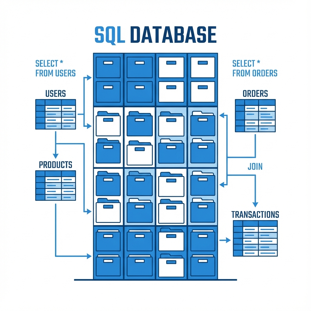 SQL (Structured Query Language) databases are like strict accountants. They store data in tables with rows and columns. Every piece of data must fit a defined structure (schema).
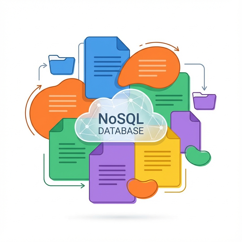 NoSQL databases are the creative artists. They are flexible and don’t require a rigid schema. Data is often stored as documents (JSON-like), key-value pairs, or graphs.
 This is where things get exciting. Vector databases don’t just store text; they store meaning. They convert data (text, images, audio) into high-dimensional vectors (lists of numbers).